2  The Utility of Mixed Models in Sports Science

2.1 Abstract

Title: The utility of mixed models in sports science: A call for further adoption in longitudinal data sets

Purpose: Sports science research consistently contains repeated measures and imbalanced data sets. This study calls for further adoption of mixed models when analysing longitudinal sports-science data sets. Mixed models were used to understand whether the level of competition affected the intensity of women’s rugby league match play.

Methods: A total of 472 observations were used to compare the mean speed of female rugby league athletes recorded during club-, state-, and international-level competition. As athletes featured in all three levels of competition and there were multiple matches within each competition (i.e., repeated measures), we demonstrated that mixed models are the appropriate statistical approach for these data.

Results: We determined that if a repeated-measures ANOVA were used for the statistical analysis in the present study, at least 48.7% of the data would have been omitted to meet ANOVA assumptions. Using a mixed model, we determined that mean speed recorded during Test matches was 73.4 m·min-1, while the mean speed for NRLW and Origin matches were 77.6 and 81.6 m·min-1, respectively. Random effects of team, athlete, and match all accounted for variations in mean speed, that otherwise could have concealed the main effects of position and level of competition had less-flexible ANOVAs been used.

Conclusion: These data clearly demonstrate the appropriateness of applying mixed models to typical data sets acquired in the professional sports setting. Mixed models should be more readily used within sports science, especially in observational, longitudinal data sets such as movement pattern analyses.

The following chapter is a copy of the published manuscript:

Newans, T., Bellinger, P., Drovandi, C., Buxton, S., & Minahan, C. The utility of mixed models in sports science: A call for further adoption in longitudinal datasets. International Journal of Sports Physiology and Performance. 17:8 p. 1289-1295.

As co-author of the paper “The utility of mixed models in sports science: A call for further adoption in longitudinal datasets”, I confirm that Timothy Newans has made the following contributions:

  • Study concept and design

  • Data collection

  • Data analysis and interpretation

  • Manuscript preparation

Name: Clare Minahan

Date: 29/03/2023

2.2 Introduction

Highly-controlled, longitudinal, or cross-over designed research experiments are difficult to conduct in the high-performance sport environment. Researchers are regularly met with hesitation from both coaching staff and the athletes due to the potential disruption ‘best-practice’ research methodology poses to competition and their carefully configured training programs. Nonetheless, to advance the understanding of performance and adaptation in elite athletes, Sports Scientists, and researchers often interrogate routinely collected health (Bartlett et al., 2020; Ferris et al., 2018; Halson, 2014), wellbeing (Bellinger et al., 2020; Gallo et al., 2017; Govus et al., 2018), physical and physiological performance metrics, and locomotive movement data (i.e., movement patterns) (Griffin et al., 2021; Newans et al., 2021; Quinn et al., 2020; Thornton et al., 2020) over multiple days, weeks, and years. Indeed, these observational studies have played a critical role in the understanding and development of sports performance and related disciplines over the last 20 years. However, these data sets are often characterized by multiple dependent observations (not only across matches and competitions, but within each athlete) and imbalanced data (e.g., athletes missing due to injuries, team selections, and/or rescheduling) that pose a significant challenge for this type of research. Nonetheless, the nuisances associated with dependent observations and imbalanced data are among the least acknowledged when conducting sports-science research.

Analysis of variance (ANOVA) with repeated measures has dominated as the most frequently utilized statistical method with which to analyse repeated measures data sets. However, ANOVA requires every participant to have a value in every observation and within a condition (e.g., position) every participant must have contributed an equal number of observations to avoid violating the relatively stringent assumptions (Kenny & Judd, 1986). Despite these assumptions, ANOVAs are still readily used within longitudinal sports science research (Hannon et al., 2021; Haugnes et al., 2019; McCaskie et al., 2019; Rago et al., 2020; Tierney et al., 2021). A systematic review of contextual factors on match running in rugby league (Dalton-Barron et al., 2020) reported that only seven of fifteen studies using the Global Navigational Satellite System (GNSS) to quantify movement patterns in athletes during match-play accounted for repeated measures within athletes (i.e., dependent observations). Of these seven, two studies eliminated data to run their ANOVA, while another study did not account for the athletes’ natural variation in performance, leaving only four studies utilising their full data set. Clearly, the characteristics of routinely collected health, wellbeing, and performance data sets in the high-performance sport environment can involve the manipulation of data, and depending on its severity, can undermine the confidence of analysis.

Obvious to the statistician and data analyst is that mixed models are likely a more appropriate statistical methodology for routinely collected health, wellbeing, and performance data such as the data in the present study. Indeed, within statistics literature, McElreath argues that mixed models deserve to be the default form of regression and that experiments that do not use a mixed model should justify not using this approach (McElreath, 2018). In his argument, he lists four reasons to use mixed models: i. To adjust estimates for repeat sampling, ii. To adjust estimates for imbalance in sampling, iii. To model variation among individuals or other groups, and iv. To avoid averaging, as some researchers pre-average data before running analyses (McElreath, 2018). Therefore, it is reasonable to suggest that mixed models are the most appropriate statistical methodology to analyse longitudinal data sets often acquired by Sports Scientists. This aligns with previous guidance by Hopkins and colleagues (2009) in encouraging sports science researchers to utilise mixed models rather than a repeated-measures ANOVA (Hopkins et al., 2009). While mixed models have become more popular within sport-science research (Bellinger et al., 2020; Newans et al., 2021; Quinn et al., 2020), the use of mixed models are often perceived as technical and requiring statistical expertise. Thus, the aim of this study was to make Sports Scientists aware of the utility of mixed models when analysing longitudinal data sets. To illustrate this, we described and compared the movement patterns of female rugby league athletes across three levels of competition. We hypothesised that match intensity, as determined by the mean speed, would be higher in Origin matches due to the higher quality players compared to NRLW matches and shorter duration compared to Test matches.

2.3 Methods

2.3.1 Subjects

Over the 2018-2019 seasons, we were provided access to athlete positioning and timing data (i.e., movement patterns) transmitted by the GNSS for Australian female rugby league athletes including: club- (i.e., National Rugby League Women’s; NRLW), state- (i.e., State of Origin; Origin), and international-level (i.e., Trans-Tasman Test; Test) competition. These data provided a unique opportunity to identify differences in movement patterns across three levels of rugby league competition previously observed in female athletes of other football codes (Andersson et al., 2010; Griffin et al., 2020). Importantly, the rugby-league data examined in the present study included repeated match data for multiple athletes which varied in number and level of competition. That is, some athletes playing NRLW played more matches than others, and some also played Origin and Test matches. This created a data set of repeated and dependent measures as well as an imbalance in sampling among athletes and competition level. Therefore, careful consideration of the statistical approach was paramount to derive meaningful conclusions.

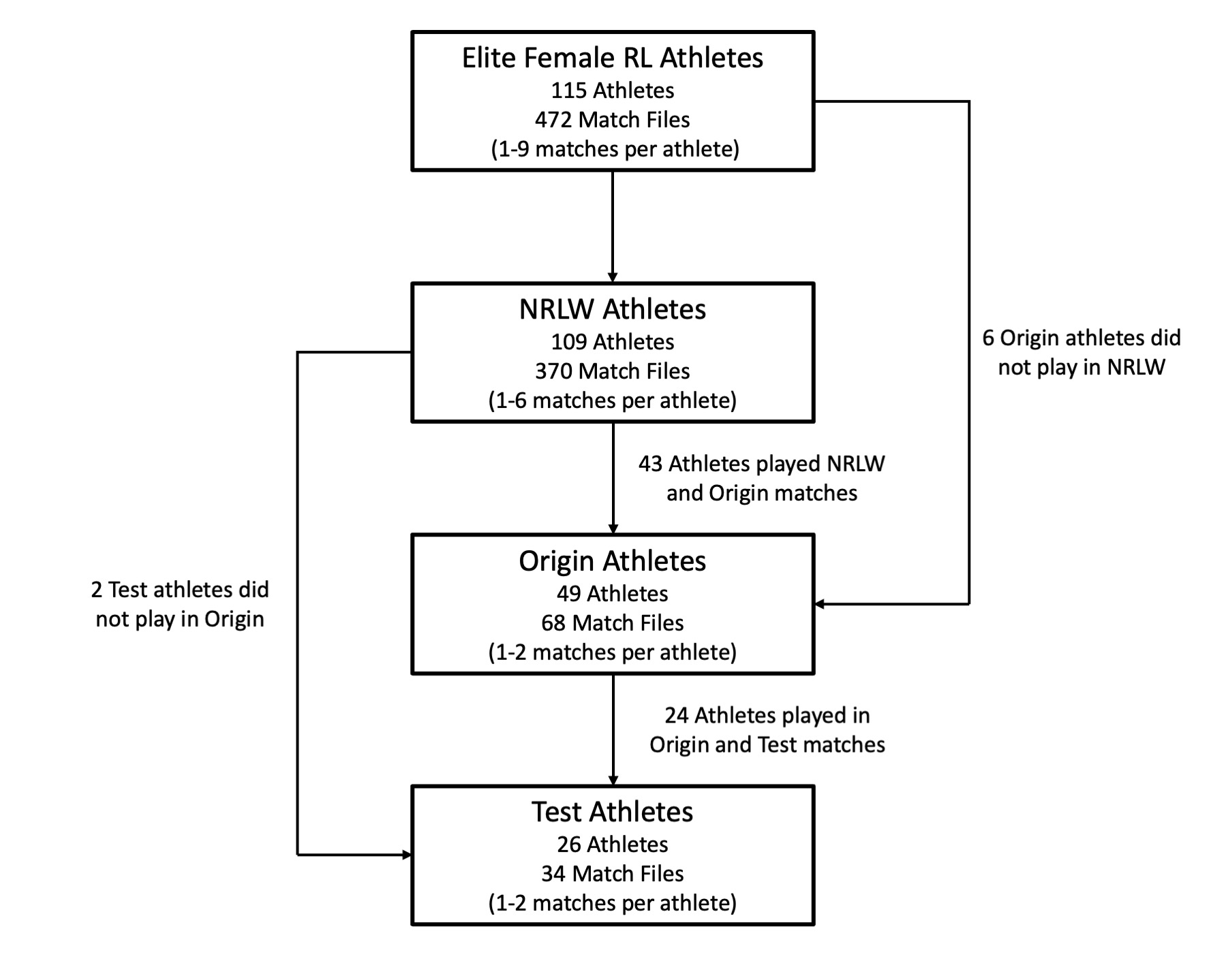
Figure 2.1 shows the sample data set that contained 109 athletes in 12 NRLW matches during the 2018 and 2019 seasons, 49 athletes in the 2018 and 2019 Origin matches (2 matches), and 26 Australian ‘Jillaroos’ athletes in 2018 and 2019 Trans-Tasman Test matches (2 matches). Collectively, the present study included 115 unique athletes (age = 26.8 ± 5.4 yr; height = 1.68 ± 0.07 m; body mass = 76.7 ± 11.9 kg) and 472 match entries.

Figure 2.1: Flowchart of women’s rugby league athletes playing at various competition levels indicating the levels of dependency within the data set. N.B. NRLW = National Rugby League Women’s; Origin = State of Origin; Test = Trans-Tasman Test.

2.3.2 Design

The present study was a retrospective, observational, cohort analysis using GNSS-derived data routinely collected by each team’s Sports Scientists. The National Rugby League coordinated the distribution of receivers, amalgamation of the data, and provision of the data sets to the authors.

2.3.3 Methodology

The movement patterns of athletes competing in NRLW matches were collected using 10 Hz Optimeye S5 receivers (Catapult Sports, Victoria, Australia), while the Origin and Test movement pattern data were collected using 10 Hz GPSports EVO receivers (Catapult Sports). To measure match intensity, the mean speed (i.e., total distance divided by the time spent on the field) of each athlete was recorded. While it was not ideal that units by different manufacturers were used, only the total distance was required for this analysis which has been found to differ by 1.8% between these two devices (Thornton et al., 2019). As the mean speed of NRLW athletes has been found to decrease as function of the minutes played, a minimum threshold of 20 min of game time was applied to ensure the athlete spent an adequate time on the field. Additionally, this filter removed athletes playing for a short duration and therefore recording a high mean speed (i.e., metres/minute) if there were no stoppages in the short time they were on the field.

Show the code:
library(lme4)
library(effects)
library(dplyr)
library(sjPlot)
library(ggplot2)
library(performance)
library(see)
library(patchwork)
library(kableExtra)
options(scipen = 999)
NRLW <- read.csv("www/data/Study_1_mm_nrlw.csv") ## Read in data
NRLW$FieldTime <- chron::chron(times = as.character(NRLW$FieldTime)) ## Turn field time into a time variable type
NRLW <- NRLW %>%
  filter(FieldTime > chron::chron(times = "00:20:00")) ## Filter only those playing more than 20 min
NRLW$MMIN <- NRLW$TotalDistance / NRLW$FieldTime / 60 / 24 ## Calculate running intensity (m/min)

Consequently, of the 472 match files, 380 were deemed eligible for analysis. The Griffith University Human Ethics Committee approved this study (GU Ref No: 2019/359).

2.3.4 Statistical Analysis

To compare the differences in analysis, both a repeated-measures ANOVA and a mixed model were fitted to the present study data set. In both analyses, the effect of a player’s position and level of competition on mean speed was assessed. For the ANOVA to be performed, we restructured the data to achieve a ‘complete-case analysis’ (Nakai & Ke, 2011). The mixed models were built using the lme4 (Bates et al., 2015) package in R version 4.0.2 (R Core Team, 2019), while the emmeans (Lenth, 2020) and sjPlot (Lüdecke, 2020) packages were used for pairwise comparisons and model diagnostics respectively. The see (Lüdecke, Patil, et al., 2021) and performance (Lüdecke, Ben-Shachar, et al., 2021) packages were used to determine which model was the best performing model. The data set was arranged in ‘long form’ with each observation for each athlete on a new row.

Show the code:
full_model <- lmer(MMIN ~ Competition*Position + (1|Player)  + (1|Team) + (1|Match), data = NRLW) ## Build full model

After loading in the lme4 package, the first model was built and the following components were outlined:

1. Dependent Variable; the metric we were interested in explaining. In this case, mean speed which as expressed as a continuous variable.

2. Fixed Effects; the variables of interest that could explain variation in the dependent variables. Here, we are looking at ‘level of competition’ and ‘playing position’. An interaction effect was also assessed, which would determine whether the difference in mean speed because of level of competition was uniform across all positions or whether the difference in mean speed because of level of competition is different for each position.

3. Random Effects; the variables that contain variation purely from the random sampling which could hide the influence of the fixed effects and would vary if the study were to be replicated (Yarkoni, 2019). Here, they are:

  1. ‘athlete’ as an individual athlete could have played up to 12 matches;

  2. ‘team’ as the team that an athlete plays for (e.g., Broncos, Roosters, QLD Maroons, etc.) could have a confounding effect and is nested within the levels of competition;

  3. ‘match’ as there is variation match-to-match in the intensity of play, perhaps due to weather, for example.

    These can be included as random intercepts and/or as random slopes, in this example, all three variables were included as random intercepts. By including these random effects, we can account for the variability associated with these effects to reveal the underlying effect of ‘level of competition’ and ‘position’ on the dependent variable.

4. Distribution Shape; in this case, the data adequately met the assumptions for a normal (Gaussian) mixed model. This example used a dependent variable (mean speed) that met the assumptions of a normal (Gaussian) distribution which meant that a simpler linear mixed model could be used in this case. However, this may not always be the case and, therefore the dependent variable may need to be expressed as a factor or percent, or log-transformed to reduce non-normality of the data (Hopkins et al., 2009). Alternatively, if there was frequency data (e.g., tackle count) or probability data, a Poisson distribution or binomial distribution respectively can be specified as the distribution family in the mixed model (using the glmer function rather than the simpler lmer function).

Once the full model (i.e., all fixed and random effects included) was established, the full model was compared to models without the fixed and random effects to assess the different model fits.

Show the code:
full_model1 <- lmer(MMIN ~ Competition*Position + (1|Team) + (1|Match), data = NRLW) ## Build model without Player random effect
full_model2 <- lmer(MMIN ~ Competition*Position + (1|Player) + (1|Match), data = NRLW)  ## Build model without Team random effect
full_model3 <- lmer(MMIN ~ Competition*Position + (1|Player) + (1|Team), data = NRLW)  ## Build model without Match random effect
reduced_model1 <- lmer(MMIN ~ Competition + Position + (1|Player)  + (1|Team) + (1|Match), data = NRLW)  ## Build model without interaction effect
reduced_model2 <- lmer(MMIN ~ Competition + (1|Player)  + (1|Team) + (1|Match), data = NRLW)  ## Build model without Position effect
reduced_model3 <- lmer(MMIN ~ Position + (1|Player)  + (1|Team) + (1|Match), data = NRLW)  ## Build model without Competition effect
model_comparison <- compare_performance(full_model,full_model1,full_model2,full_model3, reduced_model1,reduced_model2,reduced_model3) ## Compare the models' performance

When comparing models using the Akaike Information Criterion (AIC), it was determined that the full model was the preferred model as it displayed the lowest AIC. AIC was chosen as it includes a model complexity term (twice the number of model parameters) to penalise models containing variables that did not contribute to the model. The R2 and Root-Mean-Square Error (RMSE) were also reported for the reader but were not used for model selection. As the models were nested, a likelihood ratio test could also have been used.

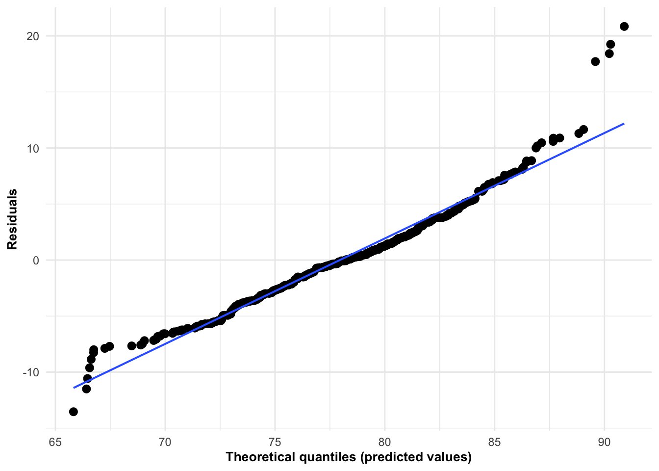
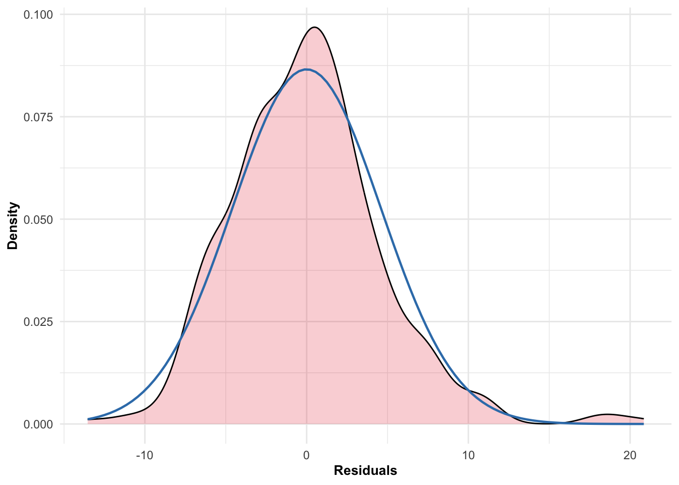
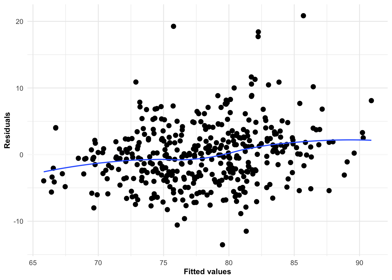
To meet the assumptions of a mixed model, a histogram of the residuals was generated to assess the normality of the residuals, Q-Q plots for each random effect were generated to assess the normality of the random effects, and the model’s residuals were plotted against its fitted value to assess homoscedasticity.

Show the code:
diag <- plot_model(full_model, type = "diag") ## Assess model diagnostics
Show the code:
plot_model(full_model, type = "diag")[[1]] +
  theme_minimal()+
  theme(plot.title = element_blank(),
        plot.subtitle = element_blank(),
        axis.title = element_text(size = 10, color = "black", face = "bold")) ## Generate Q-Q plot of predicted to residuals

Figure 2.2: Q-Q Plot of residuals for full mixed model.

Show the code:
plot_model(full_model, type = "diag")[[3]] +
  theme_minimal() +
  theme(plot.title = element_blank(),
        plot.subtitle = element_blank(),
        axis.title = element_text(size = 10, color = "black", face = "bold")) ## Generate histogram of residuals

Figure 2.3: Histogram of residuals for full mixed model.

Show the code:
plot_model(full_model, type = "diag")[[4]] +
  theme_minimal() +
  theme(plot.title = element_blank(),
        plot.subtitle = element_blank(),
        axis.title = element_text(size = 10, color = "black", face = "bold")) ## Generate homoscedasticity plot of residuals

Figure 2.4: Homoscedasticity of residuals for full mixed model.

None of these assumptions were violated so, therefore, it was deemed appropriate to proceed with the analysis.

2.4 Results

In order to meet the assumptions of a repeated-measures ANOVA, we restructured the data to achieve a ‘complete-case analysis’ (Nakai & Ke, 2011), which eliminated any athlete that did not feature in all three levels of competition. This initial filter eliminated 48.7% of the available data. Of the remaining data, each athlete varied from one to seven observations within each level of competition which continued to threaten the validity of the analysis as multiple observations of one athlete could bias the results. Secondly, it would not be suitable to answer the hypothesis as eliminating any athlete that did not play in the Test matches would result in the average NRLW mean speed being compiled of only athletes that had played in both Origin and Test matches, rather than the collective NRLW cohort. Alternatively, if we used the mean for each athlete in each level of competition, this reduced the number of observations to 157 (i.e., eliminated 58.7% of the available data). However, when averaging each athlete’s values, it would not account for the fact that there is less uncertainty in the mean speed of an athlete that had seven observations compared to an athlete that only has one observation. Therefore, it was determined that it was not appropriate to run an ANOVA across this data set. Due to the use of ANOVA being deemed inappropriate to adequately analyse these data, only the results of the mixed model are presented here.

2.4.1 Model Comparisons

Seven mixed models were assessed: the full model (i.e., containing all fixed and random effects), three models with each model removing one random effect, and three models removing the interaction effect, the competition level, and position respectively. The full model displayed the lowest AIC, the equal-highest R2, and the lowest RMSE and, therefore, was chosen as the preferred model. The results are displayed in Table 2.1. We can write the selected model in short form as:

\[ MeanSpeed_{pmti} = \beta_{0} + \beta_{1}\times Competition_{ptmi}+ \beta_{2}\times Position_{ptmi} + \beta_{3} \times \\ Competition_{ptmi} \times Position_{ptmi} + \gamma{_{p}}^{player} + \gamma{_{m}}^{match} + \gamma{_{t}}^{team} + \varepsilon_{ptmi} \]

where \(\gamma{_{p}}^{player} \sim N(0,\sigma {_{p}}^{2})\), \(\gamma{_{m}}^{match} \sim N(0,\sigma {_{m}}^{2})\) , and \(\gamma{_{t}}^{team} \sim N(0,\sigma {_{t}}^{2})\) are the random intercepts for player, match, and team respectively, and \(\varepsilon_{ptmi} \sim N(0,\sigma ^{2})\) is the residual term. All these terms are normally distributed with zero mean and variance given by the second term in the parentheses. The random effects are crossed (i.e., not nested) since, for example, a player can play for multiple teams. The model is parameterised so that the intercept term \(\beta _{0}\) corresponds to Test level of competition and the Adjustable position. Since there are three competitions and four positions in the data, the number of elements in \(\beta _{1}\), \(\beta _{2}\) and \(\beta _{3}\) is two, three and six, respectively, and are to be interpreted relative to the baseline categories in \(\beta _{0}\). Correspondingly, Competitionptmi \(\varepsilon\) {“Origin”, “NRL”} and Positionptmi \(\varepsilon\) {“Backs”, “Forwards”,“Interchange”}. Here the subscripts p, m, t and i refer to the pth player, mth match, tth team, and the ith observation for each combination of player, match, and team.

Show the code:
model_comparison %>%
  select(Name, AIC, R2 = R2_conditional, RMSE) %>%
  mutate(AIC = round(AIC, 1),
         R2 = round(R2, 2),
         RMSE = round(RMSE, 2)) ## Generate table comparing models with and without random and fixed effects
Table 2.1: Model comparison of mixed models with and without random and fixed effects.
Model AIC R2 RMSE
Full Model 2379.4 0.65 3.96
Model without Player random effect 2425.9 0.44 5.47
Model without Match random effect 2481.2 0.38 5.38
Model without Team random effect 2384.5 0.62 4.00
Model without Interaction fixed effect 2398.1 0.65 4.01
Model without Competition fixed effect 2406.2 0.64 4.01
Model without Position fixed effect 2407.0 0.64 4.03

N.B. AIC = Akaike’s Information Criterion, RMSE = Root Mean Squared Error

2.4.2 Random Effects

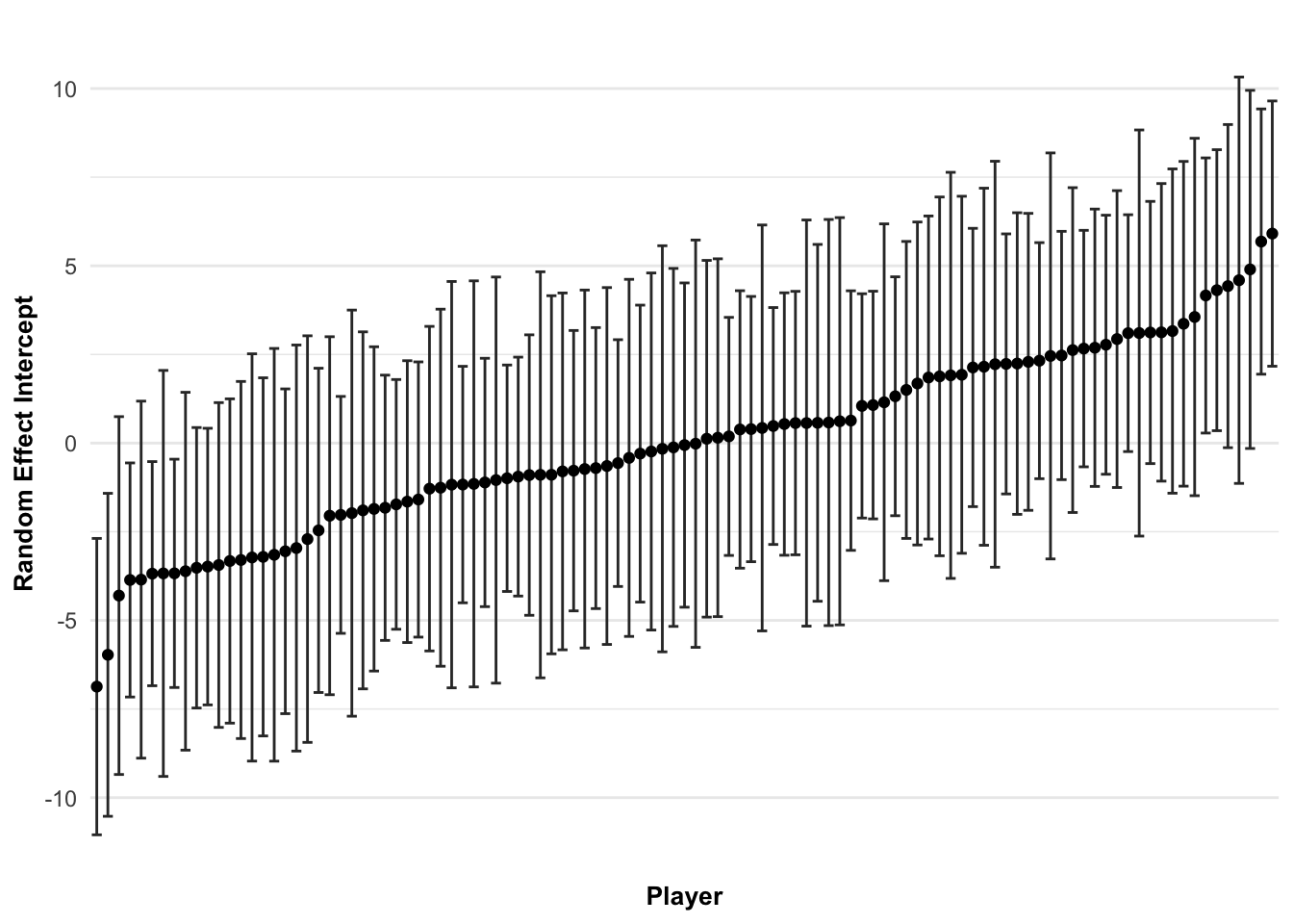
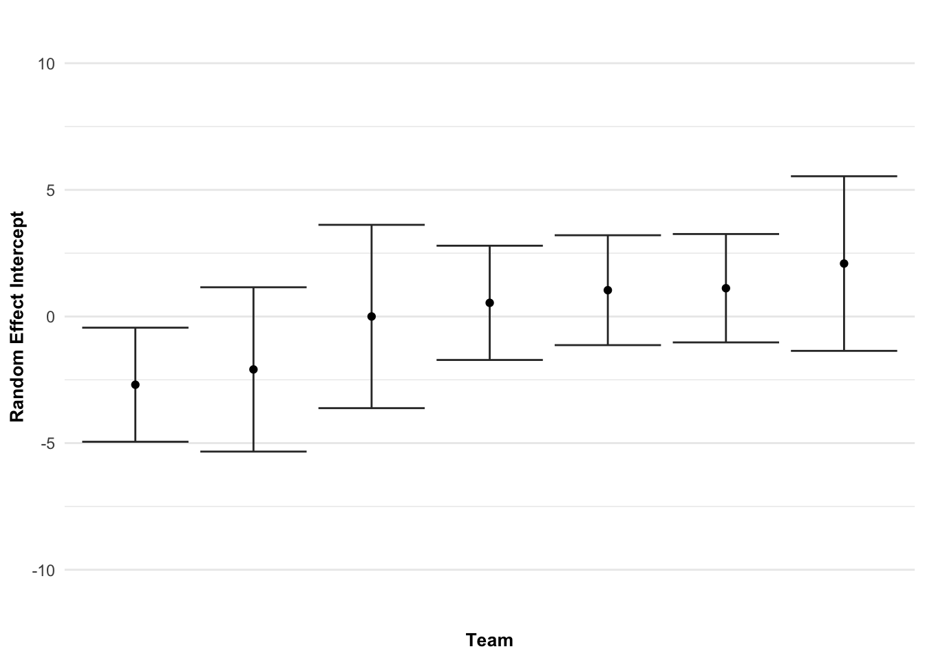
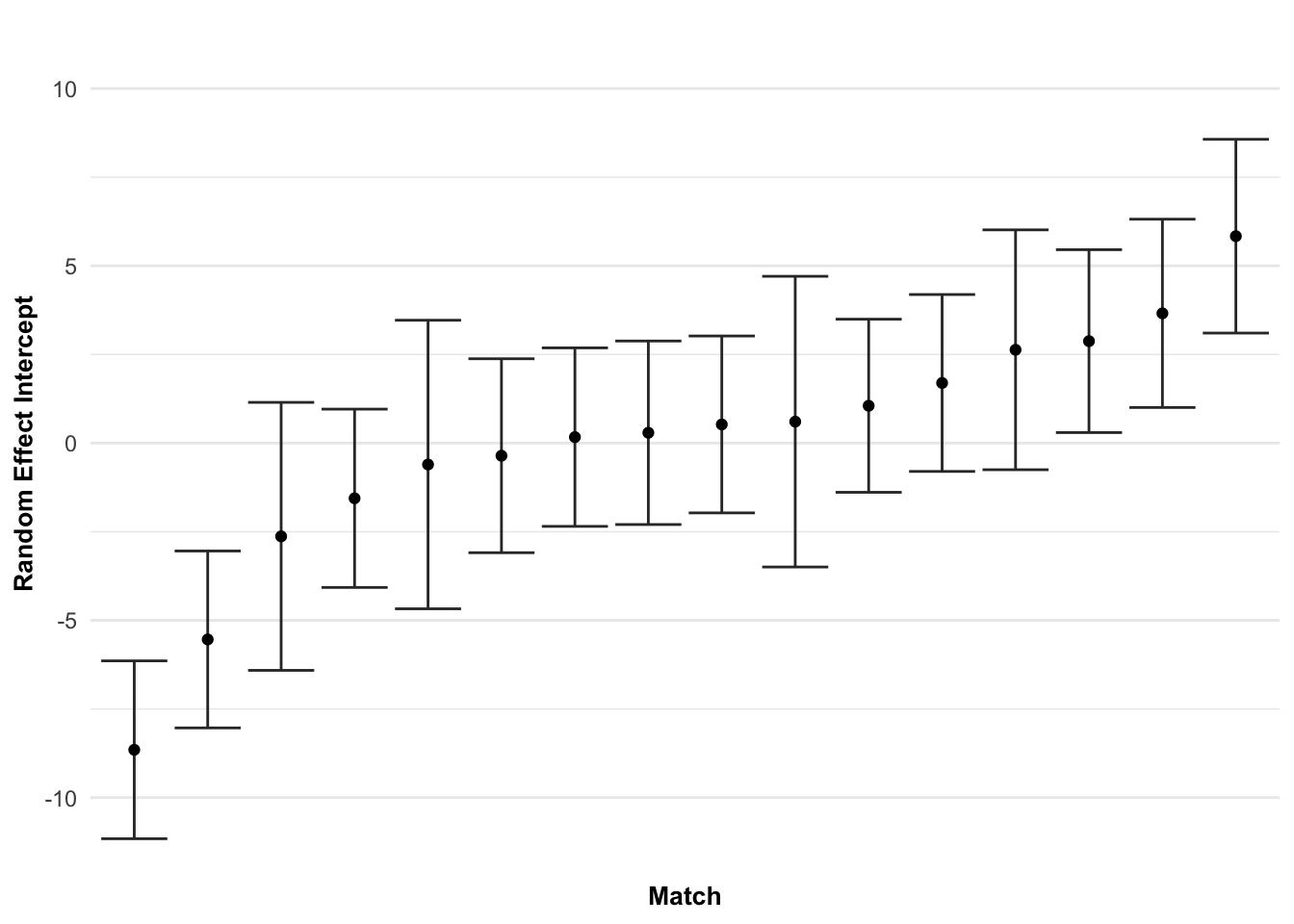
When considering the model comparison, the full model with player, team, and match random effects was preferred over the reduced models that removed each of the random effects, as evidenced by the full model having the lowest AIC value. Similarly, when assessing the variance explained by each of the random effects, it was determined that all three random effects should remain in the model. The estimated random effects variances are displayed in Table 2.2, together with the estimated residual variance. The conditional means for each level of random effect are displayed in Figure 2.5, Figure 2.6, and Figure 2.7.

Show the code:
VarCorr(full_model) %>% 
  as.data.frame() %>%
  mutate(`Variance ± SE` = paste0(round(vcov, 1), " ± ", round(sdcor, 1))) %>%
  select(`Source of Variance` = grp,
         `Variance ± SE`)  ## Generate table of random effect variances and residual
Table 2.2: Estimated variances for random effects and the model residual variance.
Source of Variance Variance ± SE
Player 13.66 ± 3.70
Match ID 14.61 ± 3.82
Team 4.31 ± 2.08
Residual 20.61 ± 4.54

The player conditional means differed between -6.9 to 5.9 m·min-1 from the marginal mean, the team conditional means differed between -2.7 to 2.1 m·min-1, and the match conditional means differed between -8.7 to 5.8 m·min-1 from the marginal mean.

Show the code:
ggplot(diag[[2]]$Player$data, aes(x = ID, y = y)) +
  geom_errorbar(aes(ymin = y - ci, ymax = y + ci), color = "#333333") +
  geom_point(color = "black") +
  scale_x_discrete(labels = NULL) +
  coord_cartesian(ylim = c(-11, 11)) +
  theme_minimal() +
  labs(x = "Player",
       y = "Random Effect Intercept") +
  theme(panel.grid.major.x = element_blank(),
        axis.title = element_text(size = 10, color = "black", face = "bold")) ## Generate Player random effect plot

Figure 2.5: Random effects for each level of player.

Show the code:
ggplot(diag[[2]]$Team$data, aes(x = ID, y = y)) +
  geom_errorbar(aes(ymin = y - ci, ymax = y + ci), color = "#333333") +
  geom_point() +
  theme_minimal() +
  scale_x_discrete(labels = NULL) +
  coord_cartesian(ylim = c(-11, 11)) +
  labs(x = "Team",
       y = "Random Effect Intercept") +
  theme(panel.grid.major.x = element_blank(),
        axis.title = element_text(size = 10, color = "black", face = "bold")) ## Generate Team random effect plot

Figure 2.6: Random effects for each level of team.

Show the code:
ggplot(diag[[2]]$Match$data, aes(x = ID, y = y)) +
  geom_errorbar(aes(ymin = y - ci, ymax = y + ci), color = "#333333") +
  geom_point() +
  theme_minimal() +
  scale_x_discrete(labels = NULL) +
  coord_cartesian(ylim = c(-11, 11)) +
  labs(x = "Match",
       y = "Random Effect Intercept") +
  theme(panel.grid.major.x = element_blank(),
        axis.title = element_text(size = 10, color = "black", face = "bold")) ## Generate Match random effect plot

Figure 2.7: Random effects for each level of match.

2.4.3 Fixed Effects

Table 2.3 displays the additive interaction effects to calculate each permutation within the data set. The intercept (i.e., 74.5 m·min-1) represents the mean speed for a Test adjustable player on average. From here, the coefficients can be added depending on what level of competition and what position was being played. For example, for the mean speed of an Origin forward athlete, you would start with the intercept of 75.0 m·min-1. From here, you will add 8.7 m·min-1 for an Origin-level athlete, then add another 1.9 m·min-1 for a forward, and then subtract 2.2 m·min-1 for the interaction effect of an Origin-level forward, resulting in an estimated mean of 83.4 m·min-1.

Show the code:
mm_fixed_effect_summary <- summary(full_model)$coef %>% 
  data.frame() %>% 
  mutate(`Fixed Effect` = rownames(.)) ## Generate fixed effect coefficients

mm_confint <- confint(full_model) %>% 
  data.frame() %>% 
  mutate(`Fixed Effect` = rownames(.)) ## Generate fixed effect confidence intervals

mm_fixed_effect_summary %>%
  left_join(mm_confint) %>%
  mutate(`95% CI` = paste0(round(X2.5.., 1), " to ", round(X97.5.., 1)),
         Estimate = round(Estimate, 1)) %>%
  select(`Fixed Effect`, Estimate, `95% CI`)  ## Compile table of fixed effect coefficients and confidence intervals
Table 2.3: Estimated means for fixed effects and interactions.
Fixed Effect Estimate (95% CI)
Intercept 74.5 (67.0 – 82.0)
Competition - Test -
Competition - Origin 8.7 (-1.1 – 18.5)
Competition - NRLW 5.1 (-2.9 – 13.1)
Position - Adjustables -
Position - Backs -2.6 (-8.2 – 3.0)
Position - Forwards 1.9 (-3.5 – 7.1)
Position - Interchange -3.9 (-9.2 – 1.4)
Interaction: NRLW-Backs -1.6 (-7.0 – 3.9)
Interaction: Origin-Backs 1.1 (-5.3 – 7.7)
Interaction: NRLW-Forwards -3.9 (-9.2 – 1.3)
Interaction: Origin-Forwards -2.2 (-8.5 – 4.1)
Interaction: NRLW-Interchange 2.2 (-3.2 – 7.6)
Interaction: Origin-Interchange -0.9 (-7.7 – 6.0)

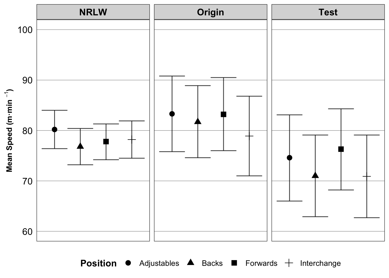
Figure 2.8 presents the estimated marginal means for mean speed recorded during NRLW, Origin, and Test matches. Origin matches recorded, on average the highest mean speed, followed by NRLW matches, and then Test matches. When considering position, in both NRLW and Origin matches, adjustables recorded the highest mean speed; however, forwards recorded the highest mean speed in Test matches. Meanwhile, backs recorded the lowest mean speed in NRLW matches, with interchange recording the lowest mean speed in both Origin and Test matches. As the changes in mean speed across competitions were not uniform across all competition, this confirmed the presence of an interaction effect.

Show the code:
Position_Estimates <- effect("Competition*Position", full_model) %>% 
  data.frame() %>%
  select(Competition, Position, fit, lower, upper) %>%
  mutate_at(vars(fit, lower, upper), round, 1) ## Create parameter estimates based on position and Competition

ggplot(Position_Estimates, aes(x = 1, y = fit, shape = Position)) +
  geom_jitter(position = position_dodge(width = 0.5), size = 3) +
  geom_errorbar(aes(ymin = lower,
                    ymax = upper),
                width = 0.5,
                alpha = .75,
                position = position_dodge(width = 0.5)
  ) +
  theme_bw() +
  scale_y_continuous(breaks = seq(60, 100, 10),
                     limits = c(60, 100)) +
  facet_wrap( ~ Competition, ncol = 3) +
  labs(y = bquote(bold('Mean Speed (m·min ' ^ -1 * ')'))) +
  theme(
    panel.grid.major.x = element_blank(),
    panel.grid.minor.x = element_blank(),
    panel.grid.major.y = element_line(colour = "grey50",
                                      linewidth = 0.2),
    panel.grid.minor.y = element_blank(),
    axis.ticks = element_blank(),
    axis.title.x = element_blank(),
    axis.text.x = element_blank(),
    axis.title.y = element_text(size = 10, color = "black"),
    axis.text.y = element_text(colour = "black", size = 12),
    strip.text.x = element_text(colour = "black", size = 12, face = "bold"),
    legend.position = "bottom",
    legend.title = element_text(colour = "black", size = 12, face = "bold"),
    legend.text = element_text(colour = "black", size = 10) ## Generate marginal mean plot for mean speed
  ) 

Figure 2.8: Mean speed of women’s rugby league athletes by competition level and position. N.B. NRLW = National Rugby League Women’s; Origin = State of Origin; Test = Trans-Tasman Test.

2.5 Discussion

The present study displayed why mixed models should be the more heavily-adopted when analysing sports science field-based data sets with repeated measures, like the rugby league women’s data set used in this study. Mixed models were able to account for multiple observations of the same individuals in the data set, players changing positions between matches, and account for inter-player, inter-match, and inter-team dependencies to extract the true effects of position and level of competition on mean speed and the appropriate quantification of the uncertainty of these estimates. One strength of the mixed model in analysing data was its ability to account for the differing number of observations of athletes. In the data set, athletes ranged between one and nine matches played with 24 athletes playing only one match, while five athletes played nine matches each. This is not ideal when applying repeated-measures ANOVA as either some athletes or some time points (i.e., games) would need to be excluded from the analysis. While removing an athlete if they do not have an observation in every time point or removing a time point if many athletes are missing is statistically appropriate if the missing data points are proved to be missing completely at random (i.e., no bias in missing data) (Borg et al., 2021), this method can cause unnecessary deletion of large amounts of data. If there are many participants and many time points, it can sometimes eliminate so much data that no analysis can be performed on the remaining data set; for example, 48.7% of the data collected for the present study would have been omitted when filtering out players that did not participate in Origin or Test matches. However, mixed models can attribute a level of uncertainty to each athlete dependent on their sample size and, therefore, the model can more accurately quantify the true mean speed of a player with nine observations compared to a single observation of another athlete. In doing so, mixed models create flexibility in the data sets that can be utilised that more closely align to data sets seen in sports due to injuries, squad selection, and access to athletes on a given day. The mixed model provided an analysis that could retain all available data points and did not require the elimination of data points to retain a ‘complete case analysis’ data set (Nakai & Ke, 2011), nor did it require data imputation to estimate missing data (Borg et al., 2021).

Another strength of the mixed model was its ability to use the dependency within the data set to increase the power of the statistics, rather than detract like in general linear model applications. For example, in the present study, since there were only two matches at an international level and only two matches at Origin level, these sample sizes would be underpowered when using a linear model; however, when merged with the twelve NRLW matches, the model can draw on the variance attributed to players and positions to estimate the effects of level of competition more robustly. Similarly, two players played in three of the different positional groups which would typically require the athlete to have matches in which they were not in their ‘primary’ position to run parametric general linear models. However, this information is actually very useful as it enables the model to observe the same athlete, in the same team, in the same level of competition but in a different position which provides more information than if the two positional groups were completely independent of each other. That is, by enabling players to be their own control group, they can more accurately interrogate the between-position differences in mean speed. As a result, mixed models can more accurately and more robustly determine the variation attributable to athletes, time points, and conditions (e.g., position) much more than any general linear model. Additionally, by using a mixed model, it was evident that the random effect for player is larger than the fixed effect of position, which would not be able to be established when using a repeated-measures ANOVA. Therefore, this reinforces that individualised training for an athlete, rather than the position, is more important from a training prescription perspective.

When considering the findings of this study, the reduced overall mean speed recorded for the Test (80 min), compared with the Origin (60 min) and NRLW (60 min) matches in the present study could be explained by the longer Test-match duration. We have previously reported that the mean speed when travelling >12 km·h−1 of athletes recorded during international matches declines by ∼40% within the first half of the match (Quinn et al., 2020). We also previously demonstrated that there were no significant differences in the relative distances covered in any of the speed zones, as well as the overall mean speed when comparing the first and second half of NRLW matches (Newans et al., 2021). These results contrast with those seen in other codes, with significantly increased total distance and high-speed running in international football compared to domestic football (Griffin et al., 2020). On closer examination of mean speed in the present study, it was evident that the position contributed to the model with forwards recording the highest intensity and the interchange athletes delivering the lowest intensity. This could be due to a disparity in playing ability between the starting forwards and the interchange replacements. We previously established that the mean speed of interchange athletes significantly reduced as their playing duration increased (Newans et al., 2021), which could explain why at the international level, when interchange athletes are required to play increased minutes due to the longer format, they cannot sustain the same intensity as the starting forwards.

2.6 Conclusion

The requirement to account for repeated measures and imbalanced data is pertinent in longitudinal sports science data sets. As previous studies have demonstrated a lack of statistical literacy to correctly understand dependency within data sets and the consequent violations of parametric statistical assumptions, the present study provides a more thorough account of the process, the associated R script, and the resultant interpretations to inform Sports Scientists on mixed models. It is anticipated that the present study will empower Sports Scientists to assess the various dependencies more critically within their data sets.

2.7 Practical Applications

  • Mixed models should be a more-heavily adopted statistical method for analysing sports science data sets with repeated measures as they are more flexible than repeated-measures ANOVA

  • Mixed models can accommodate differing frequency of observations of athletes and players swapping positions in between matches

  • If Test matches continue to be 80 min in duration, the physical and physiological capacity of athletes should be improved to maintain running intensity at the international level

  • NRLW matches should be increased to 70 min in 2022 to gradually bridge the gap between domestic- and international-level competition